A brief study of pinhole diffraction

Introduction

In this mini-project, I studied the diffraction of a HeNe laser beam through a 150 micron pinhole. I profiled the resulting Airy pattern with a photodiode, fit the data using an intensity equation proportional to a Bessel function in Mathematica, practiced imaging the pinhole at various distances with different focal-lengthed lenses, and observed the effect of using a high pass spatial filter to alter the image. I also spent some time understanding how the Airy diffraction pattern is the Fourier transform of the circular pinhole.

Profiling the Airy Pattern

We first practiced profiling the laser beam with a photodiode (connected to an AVO meter with a 100 ohm resistor) placed in the line of the Airy pattern. We started by sweeping the intensity of the center bright spot of the pattern on a moveable stage. At first the results we were getting seemed off—the sides of the center beam were Gaussian-esque, however the center seemed to just plateau at a constant value. Dr. Noé explained that the hole of the photodetector was too wide to make a fine measurement of the intensity across the small light spot. It turns out we had been measuring a convolution of the wide hole and the Gaussian shaped intensity of the beam, which (according to Fourier mathematics) appears as a square pulse with rounded edges. He also suggested that we use a much stronger resistor to make the AVO meter more sensitive to small changes in the intensity. So now with a 200-micron pinhole covering the photodiode and a 10 M ohm resistor in place of the other, we set to work at charting the intensity (in millivolts) across the central bright spot of the Airy diffraction pattern.

After becoming more comfortable with the process, we then decided to collect additional data points in order to more clearly see what’s going on in the wings of the graph. This time we collected intensity information from the n=3 diffraction fringe on one side of the center bright spot to the n=5 diffraction fringe on the other side (the unsymmetrical data collection is due to the positioning constraints of the photodiode on the moveable stage). The enter Airy disk was 11 mm in diameter and the diameter across 5 bright rings was about 50 mm.

Modeling with Mathematica

With Mathematica, we first fit a Gaussian function to the data, found the parameters for the equation (height, width, and central position), and then graphed the data points and Gaussian curve on the same axes. While the Gaussian fit obviously couldn’t account for the plurality of lesser-intense concentric rings, it appeared to be a fair estimation of the intensity of the central disk. But then after fitting an equation proportional to a Bessel function to our Airy pattern intensity data, we realized right away that it was a more suitable fit than the Gaussian one. The left figure below shows the transverse intensity data (blue points) with the Airy pattern intensity equation curve (green).

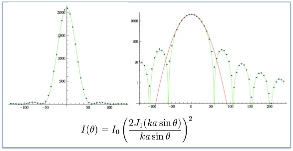
This function takes into account the aperture diameter, wavelength of the laser, and angular radius from the pattern maximum. Afterwards, we also plotted all three of these curves (blue points: data, green curve: Bessel function fit equation, red curve: Gaussian fit equation) on a semi-logarithmic plot (see right figure above). It was clear instantly that the data for the center Airy disk did not behave like the Gaussian curve, which was parabolic on these axes.

Imaging the pinhole

We then experimented with different lenses to see the distances at which we could focus the Airy diffraction pattern back down to create an image of the pinhole (using the setup as seen in the figure below). For each configuration, we used the thin lens equation to relate the reciprocals of the distance of the object to the lens, the distance of the image to the lens, and the distance of the focal length. And in each case, the results were fairly accurate.

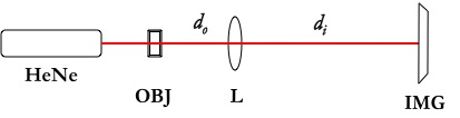
For instance, with the BSX085 lens (f = 20 cm): the object was 28 cm away, the image 68 cm away, and the sum of their reciprocals was 0.0504 cm^-1, very close to the focal length reciprocal of 0.05 cm^-1. The magnification equation revealed that the pinhole was magnified 2.43 times, (meaning its image was 364-microns). By changing the object to lens distance slightly, we observed the following: the object was 21.5 cm away, the image was 365.76 cm away, so therefore the thin lens equation yielded a sum of 0.04924 cm^-1, which is still close to the 0.05 cm^-1 reciprocal focal length.

Afterwards we tried sending the diffraction pattern across the length of the lab and projected it onto the main door (which was 1317 cm from the pinhole). We used different lenses at varying distances in the setup to try to focus the image of the pinhole onto the door across the lab. We achieved this with the BSX085 lens (f = 20 cm) at a distance of 21.6 cm from the object and 1295 cm from the image. Using the lens equation, the sum of the distance to object and to image reciprocals was 0.047 cm^-1, relatively close to the actual focal length reciprocal of .05 cm^-1. The magnification equation with these distances resulted in a magnification of 60 times, which means the calculated image height was 9 mm. We measured that the actual crisp-edged pinhole image had a diameter of about 11 mm.

Fresnel Diffraction Patterns

When we took another look at the Airy pattern and the image in focus at the opposite side of the lab, Dr. Noé showed us how you could see the Fresnel diffraction patterns as you move a piece of paper closer to the lens to observe the transverse plane of the beam. At a certain distance, there was a dark spot in the middle of a light ring, then a light spot in the center, etc. This pattern was what the lens was imaging right in front of the pinhole, and it alternated until you reached the image of the Fraunhofer diffraction zone.

We then saw something unexpected, which was that when we moved the paper farther than the focused pinhole image, out of the lab to the wall across the hall, we noticed the same alternating Fresnel patterns again. These patterns were what the lens was presumably imaging on the other side of the pinhole? But we weren’t exactly sure and had to do a little extra research.

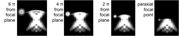
We found this article that actually explains why we were seeing different patterns over a certain distance behind the focused image of the pinhole. Evidently with pinhole aperture diffraction, the classic Airy pattern is only present at the point of paraxial focus, in other words the intermediate image plane. The article contained an axial intensity distribution plot (figure above) that showed why we were observing the dark-center diffraction pattern at certain distances; there was also a helpful demo to click through for a transverse representation of the diffraction pattern at each of those distances (figure below). I thought it was also interesting to note that there were more higher-order diffraction rings at a distance ±6π from the point of paraxial focus than there are in the classic Airy pattern at this paraxial focus point.

Understanding Spatial Frequencies

In a diffraction pattern, the high spatial frequencies contain information about the edges and details of an object, while the low spatial frequencies contain information regarding the overall quality of the object.

The spatial frequency is the reciprocal of the wavelength, so in other words it is the rate of change in space. Therefore, if we were to think of an object as a 2D picture, at an edge where there is a more abrupt change, there is a steeper gradient. For instance, the edge detection technique used in image alteration makes use of this and finds the steepest gradient between neighboring pixels. On other areas of the object where there is no (or very slight) variation between pixels, the gradient would be zero (or very close).

With a pinhole, light propagating through has to bend at a greater angle at the edge of the aperture. If a lens is placed one focal length away (as seen in the setup below), these rays will be focused by the lens to the outer sections of the diffraction pattern in the Fourier plane. In the center of the aperture where light is transmitted unbent, the light rights will be focused to the optical axis in the center of the diffraction pattern. So the Airy diffraction pattern in the Fourier plane is the Fourier transform of the pinhole: it’s a description of the aperture in terms of its spatial frequencies.

By altering the diffraction pattern in the Fourier plane, we can alter how the pinhole will be imaged. Since the high spatial frequencies contain information regarding the edges of an object, we assumed that by adding a high pass filter we would see the pinhole image with a sharper border and maybe a darkened center.

High Pass Filter

We then put a high-pass filter into the setup in order to see the effect on the image. We created a circle of whiteout on a piece of transparency, but no matter how uniform the circle looked to the eye, once we placed it in the setup in front of the beam of light the shadow it created revealed the whiteout shape’s uneven edges..

We configured the setup so that the pinhole image would be magnified enough for us to observe the effect of the filter. The image was similar to what we had expected: there was a bright circular ring of light with a dim inside, but it also seemed messy inside- with an extra softer ring of light and some speckle outside. This was probably due to the irregular shape of the filter and maybe some kind of aberration effect from the transparency sheet.

Conclusion

The mini-project allowed me to explore the basic optics principles behind the 4-f spatial filtering setup, namely diffraction theory and Fourier optics, which I then used to create Bessel-like beams for my main research project.