Introduction

As a sophomore at Juniata College, I was enrolled in an advanced course in microscopy where I took immediate liking to the subject. Although interested in the biological applications of the field, I was actually drawn in by the optical characteristics of the involved instrumentation. Upon arrival at the Laser Teaching Center, I hoped to work on a project that would incorporate my interests in microscopy with optics research. By chance, I was introduced to Dr. Jonathan Sokolov of the Garcia Center who utilizes modern microscopy techniques to image DNA and other polymers. He was generous enough to allow me to collaborate with him on his current research project involving confocal imaging of DNA.

This photo is from my initial visit to the Garcia Center.

The overall goal of Sokolov's immediate research, discussed in detail below, is to determine specific alignments of fluorescent tags when bound to single and double stranded DNA using confocal microscopy. Due to the restriction of integrated microscope laser systems, an off-axis illumination system needed to be designed for effective tag excitation and sample illumination/imaging. A 473 nm diode-pumped solid-state (DPSS) laser was chosen as the illumination source. My task as a collaborator on this project was to characterize (determine) the output power, polarization, and beam profile of the laser as a function of control voltage and, under certain circumstances, distance (z) from the face of the laser. The information will be useful in maximizing the effect of off-axis illumination on the biological sample.

Project Goal

Sokolov's immediate research is focused on viewing the binding orientation of fluorescent tags when attached to DNA. The tags used in the project, YOYO-1, Acridine Orange, and SYBR Gold, are largely polarization dependent. When these tags bind to DNA, they do so differently, depending upon the nature of the polymer. In single stranded DNA, the tags are expected to cling to the phosphate backbone due to electrostatic interactions, whereas in double stranded DNA, the tags are expected to intercalate (rest between nucleotide base pairs) due to hydrogen bonding. Orientations can be distinguished using certain fluorescence microscopy techniques. Confocal microscopy, for instance, is a technique that is capable of imaging several optical sections ("z" series) of the specimen and constructing a three-dimensional representation from them using special computer software [1]. At the Garcia center, a laser scanning confocal microscope (LSCM) is used to assist in the imaging of fluorescently tagged specimen, especially DNA. This specific instrument is equipped with three laser systems integrated into the optical train to serve as illumination/excitation sources. Although the feature is largely convenient, integration severely limits the ability of the researcher to alter both the polarization of the laser beam and its angle of incidence upon the specimen. This was a major setback in Sokolov's research, as the limitations of the microscope made it almost impossible to distinguish between tag binding orientations of the polarization dependent dyes. Fortunately, by the imposition of specific illumination techniques, the visualization issues can be combated. Oblique illumination, for instance, offers increased resolution and contrast in imaging microscopic specimen by restricting light to off-axis positions at specific angles [2]. This technique was tested on the Garcia center LSCM using an ordinary, fluorescent lightbulb, showing radical improvement in image quality. The lightbulb was not properly polarized to maximize fluorescence/specimen excitation, so to increase the effectiveness of the technique, a 473 nm diode-pumped solid-state laser was purchased for use as an illumination source. The wavelength of this laser, 473 nm, is appropriate for excitation of the fluorescent tags used in the experiment. (Tag excitation peaks range from 491 -- 502 nm). By mounting the laser on an adjustable stage, the excitation source will be able to be manipulated to achieve specific illumination angles. In addition, the polarization of the laser will be able to be adjusted by a half-wave plate on rotational mount, placed in the path of the beam.

The DPSS Laser

Our laser (Fig. 1), model DHL-B50N from Ultralasers, Inc., is similar to a common green laser pointer. The pointer beam is created using an 808 nm diode laser to pump a Neodymium-doped Yttrium Aluminum Garnet (Nd:YAG) or a Neodymium-doped Yttrium Orthovanadate (Nd:YV04) crystal. The crystal produces a 1064 nm beam which is then frequency doubled by a non-linear crystal -- Lithium Triborate (LBO) or Beta Barium Borate (BBO) -- to 532 nm, producing a bright green beam. The blue DPSS laser, like the green laser pointer, uses an 808 nm diode pump laser and a non-linear crystal for frequency doubling. Unlike the laser pointer, the Nd:YAG crystal in the blue laser is set up so that the beam undergoes a weaker wavelength transition to only 946 nm. After frequency doubling, a rich blue beam is produced.

         

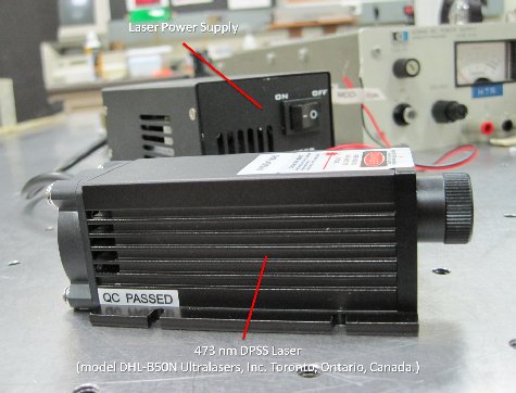
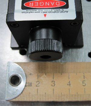
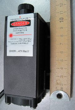
Figure 1: The DPSS Laser. Images of the DPSS laser revealing its compact size.

Output Power and Polarization

The blue DPSS laser receives its input power from a normal 120 V AC wall outlet, yet its output power can be modulated by a second input, used to deliver a 0 -- 5 V DC control voltage (V_c). Output power versus V_c was measured using a thermal power meter(Scientech Model 365 with Type 360001 detector head) in 0.5 Volt increments from V_c = 0.5 -- 5.0 Volts. Power was just 1.35 mW at V_c = 0.5 Volts and approximately doubled for each increment up to 4.0 Volts, leveling off at 110 mW (Fig. 2). After later discovering that beam quality degrades dramatically at Vc < 2.0 Volts, we conclude that the laser can operate at a power output range of ~ 16 -- 110 mW (V_c = 2.0 -- 4.0 Volts) with acceptable beam quality.

         

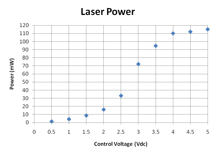
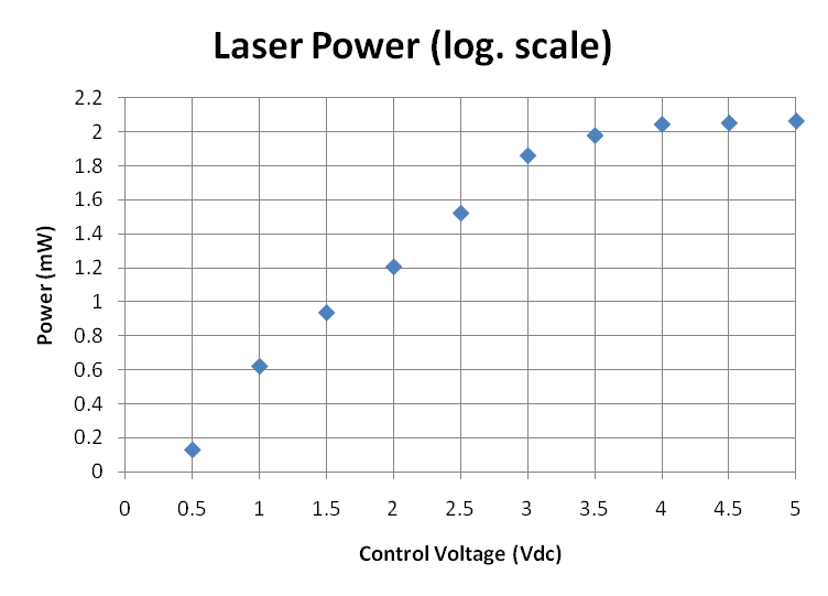
Figure 2: Output power versus control voltage. Click on either graph to display a larger image.

Polarization was determined by shining the DPSS laser beam through a Glan-Thompson polarizer and into a photodetector. The polarizer was rotated to find the maximum and minimum current at different control voltages. Extinction ratios were determined for specific control voltages by dividing values of transmitted light readings at maximum by those at minimum. The polarization was found to be vertical in nature (with respect to the laser body). At its maximum control voltage (5 Volts), the extinction ratio of the laser was determined to be only 35:1, significantly lower than the quoted extinction ratio of 100:1 [3]. As the control voltage was lowered, the extinction ratio also decreased, proving to be as low as 1.5:1 at V_c = 2.0 Volts.

Beam profile -- Theory

The most extensive part of the project involved determination of the profile, or shape, of the beam. This can be determined using several methods. In this experiment two have been utilized, the first involving the comparison of experimental data to a theoretical Gaussian curve. This curve, denoted by the equation I = I₀e^{-2r2⁄ w2}, explains the intensity of the laser beam, where r = distance from the beam waist, and w = beam radius at distance r [4]. It shows that in a perfect Gaussian, the intensity of the laser should be the greatest at the center of the beam and drop off evenly moving in any lateral direction away from that point. When data is superimposed over a theoretical curve, the quality of the laser beam can be determined by the fit of the points. Also, the waist (radius) of the beam can be found as a function of 1/e². At this point, r is equal to w and the intensity is approximately 14% of the maximum intensity [4].

The second method used to profile the beam involves the determination of beam divergence. Waist size at specific distances, z, from the face of the laser can be found using the equation w(z) = w₀[1 + (^z⁄z_R)^2%frac12; where z_R, the Raleigh range, is equal to ^λw2₀⁄π [4]. A theoretical curve proves to be hyperbolic in nature. When z is much greater than z_R, the equation becomes linear, as only the initial waist (w₀) and the distance from the waist are taken into account. When z is much smaller than z_R, all aspects of the equation must be taken into account. This shows that at far distances from the laser, the beam diverges at a much faster rate than at close distances. By fitting a theoretical curve to experimental data, initial waist size w₀ of the tested beam can be determined. Using this value, the full angle divergence of the laser beam can be calculated using the equation θ = ^.637λ⁄w₀ [4].

Beam Profile -- Experiment

In order to obtain data to compare to the previously stated theoretical equations, several experiments were conducted. The first involved a razor blade mounted on a translation stage used to "slice" through the DPSS laser beam pointed at a detector. Intensities were recorded in microamps and milliwatts, depending upon the detector being used (photodetector or thermal power meter). Current readings were performed at six distances from the face of the laser up to approximately one meter at V_c = 2 Volts. Power readings were performed for V_c = 2, 4 Volts at two distances within 0.3 meters. Intensities were plotted as a function of lateral distance across the path of the laser beam (Fig. 3). Graphs show that beam intensity drops off as a function of distance sliced into the beam, plateauing as the razor approaches spot edges. The initial waist of the laser (w₀) was estimated from each of the plots.

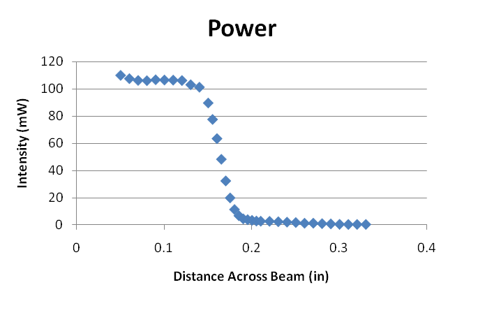
Figure 3: Razor Blade Experiment. Graphs demonstrate the intensity of the Gaussian profile at specific lateral distances across the path of the laser beam. Both show the intensity of the beam changing rapidly at the beam center, but begins to level-off or plateau at the beam edges. The leftmost graph is a representation of the beam intensity in terms of μA. The rightmost graph is a representation of the beam intensity in terms of mW.

The second profiling method involved the use of a 100 μm pinhole mounted on a translation stage to scan across the path of the laser beam. (The beam intensity was maximized at the center of the pinhole preceding each set of measurements). This technique was first utilized to measure intensity in terms of microamps at six distances up to approximately 1 meter (V_c = 2 Volts). To increase the sensitivity of measurements, readings were later taken in terms of millivolts. The voltage method was used to experiment at eight distances from the laser face up to approximately 3 meters at V_c = 2, 3, 4 Volts. It was also used at six distances, up to approximately 1 meter, at V_c = 1 Volt. At V_c = 1 Volt, data fit poorly to the theoretical curve (Fig. 4), but with increasing V_c (at 2, 3, 4 Volts) and increasing distance from the laser face, data was better suited to the curve (Fig. 4). Waists were determined for each data set. In addition to these experiments, the method was also conducted at 7.92 meters using a 1 mm pinhole and a photodetector where V_c = 2, 4 Volts. Data fit well to a theoretical Gaussian curve at this distance (Fig. 5). For each data set, beam waist, as a function of ¹⁄e², was determined.

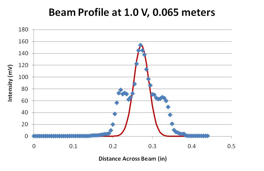
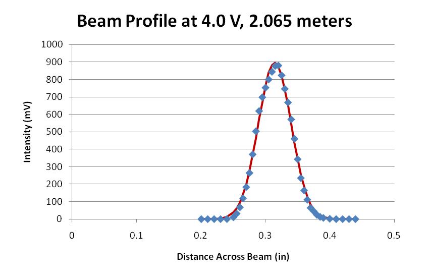
Figure 4: Gaussian Distributions (≤3 m). Plots demonstrate beam intensity distributions in terms of mV using the pinhole method. The leftmost plot depicts the Gaussian profile of the beam at 1.0 Volt, at the closest distance to the laser face (0.065 m). Comparison of the experimental data to the superimposed theoretical Gaussian curve proves a poor fit. The rightmost plot depicts the Gaussian profile of the beam at 4.0 Volts, at the further distance from the laser (2.065 m). Experimental data shows a dramatically improved fit to the theoretical Gaussian curve when compared against the plot at 1.0 Volt, 0.065 m.

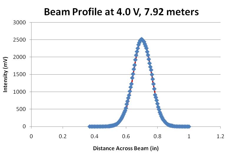
Figure 5: Gaussian Distributions (7.92 m). This plot demonstrates beam intensity distribution in terms of mV as in Figure 4. The experimental data (4.0 Volts, 7.92 m) fits well to the superimposed theoretical Gaussian curve as in the 4.0 Volt plot at 3.65 m.

The third method used to profile the laser beam was a visual determination of spot diameter. Surprisingly, the laser was found to produce an elliptical spot (Fig. 6). All previous measurements have been confined to the long, horizontal axis of the laser beam. Measurements of beam diameter were taken at V_c = 2 Volts for specific distances from the face of the laser up to 26 meters. Data was plotted as a function of spot radius (waist size) and distance from the laser against a theoretical curve in order to determine the initial waist size w₀ (Fig. 7). To determine the full angle divergence of the beam, the equation θ = .637*λ/w0 was used [4]. The resulting divergence was determined to be 0.6 mR, differing from the maximum quoted divergence of 1.2 mR [3] by a factor of two. The initial waist of the laser beam was found by plotting experimental data from all three methods against a theoretical hyperbola. This value was determined to be approximately 470μm, corresponding to a spot diameter of 940 μm (on par with the quoted diameter of approximately 1.0 mm [3]).

Figure 6: Beam Spot Visualization. This image is a photograph of the DPSS laser beam spot at approximately 26 meters. It is elliptical in nature, having a long horizontal axis and a short vertical axis with respect to the laser body.

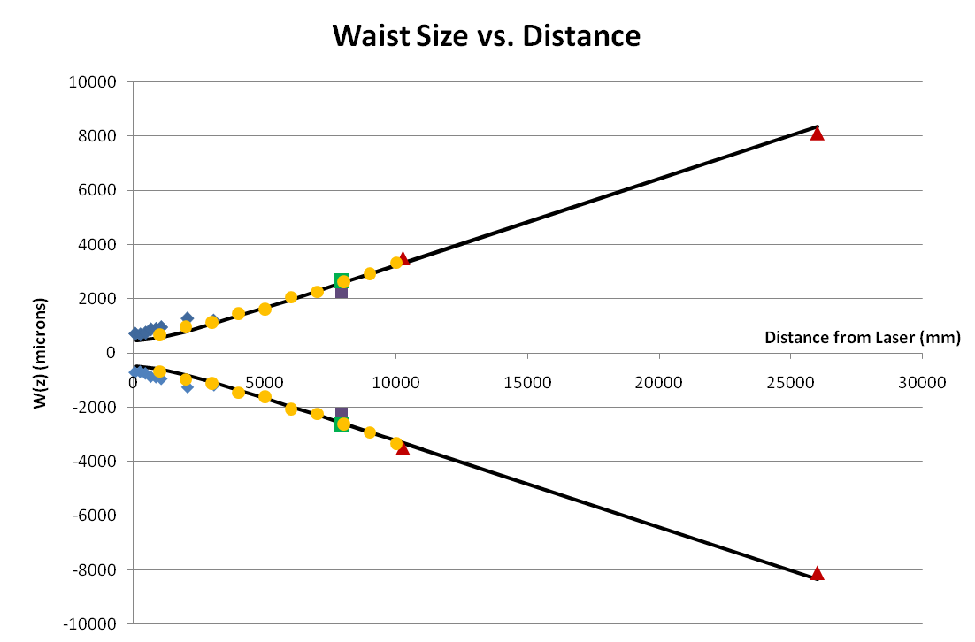
Figure 7: Beam Divergence. This plot contains waist divergence data from two of the three profiling methods, plotted against a theoretical curve that assumes a waist of 470 μm. Blue and green marks are representative of pinhole data. Visualization data is represented by purple, yellow, and red marks. Divergence proves to be small at distances close to the initial waist. The data shows greater divergence at further distances from the face of the laser.

Conclusion

Overall, the DPSS laser proves to operate with acceptable beam quality over a power range of approximately 16 -- 110 mW. Its initial waist is approximately 470 μm, yet the beam spot is elliptical in nature, so this is only a calculation of the long, horizontal axis of the beam. The divergence is only approximately half of the quoted value for reasons currently unknown. Although the polarization was poorer than expected, decreasing/low extinction ratios may be combatted with the use of a polarizer. Unfortunately, this may cause other problems with beam intensity and proper tag excitation.

Future experimentation should involve characterization of the beam in a vertical orientation with respect to the laser body. This should give insight into the effect of the elliptical nature of the beam and may account for discrepancies in quoted and experimental values. Other methods of beam characterization may be employed to further understand the nature of the DPSS laser. Tag excitation is currently underway, but resulting confocal images have not yet been analyzed for tag binding orientation. With this analysis, the success of the oblique laser illumination/excitation can be understood and, from there, mechanically manipulated or optically altered to enhance the effectiveness of the technique.

Acknowledgements

I would like to thank Drs. John Noé and Marty Cohen for their guidance throughout the course of the project, as well as their assistance in data analysis and troubleshooting. I would also like to thank Dr. Jonathan Sokolov for allowing me to be part of his research group and for his assistance in understanding the biological aspects of this project. In addition, thanks goes to Ashish Sridhar and Suri Bandler for their assistance in the polarization portion of this study. This project was made possible by financial support from NSF Grant PHY-0851594 and the Laser Teaching Center, and to both, much thanks is given.

References

[1] Fellers T J, Davidson M W. 2010. Introduction to Confocal Microscopy. Olympus Microscopy Resource Center. . Accessed 2011 June 27.

[2] Abramowitz M, Spring K R, Fellers T J, Davidson M W. 2010. Oblique Illumination. Olympus Microscopy Resource Center. . Accessed 2011 June 16.

[3] [Ultralasers, Inc.]. 50 mW 473 nm DPSS Lasers. Ultralasers, Inc. 2011. . Accessed 2011 July 5.

[4] Hecht E. Optics. Boston (MA): Addison-Wesley; 2001. 698 p.

[5] Goldwasser S M. 2011. Diode Lasers. Sam's Laser FAQ. . Accessed 2011 July 10.