Introduction

First, before reading this, it may be valuable to read some background data from my weblinks page. Specifically, look at the links under the the Fiber Optics heading. Also of interest are the Hollow and Exotic Beams and the General Physics, Optics, and Math sections.

A fiberoptical cable is a cable that is capable of carrying light with generally low losses. Modern cables have a core, made of glass, and cladding, made of some other material whose properties (specifically index of refraction) make it suitable for use. Fiberoptical cables are widely used in computer networking, where square pulses of light are used to represent digital 1s and 0s. In the cable, these square pulses suffer attenuation and flattening, so over long distances the signal must be periodically read and retransmitted. The type of cable used in computer networking does not keep the light rays in their original orientations with respect to each other.

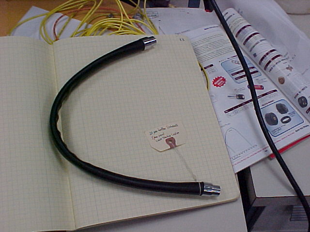
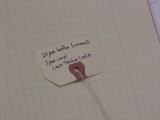
However, if several fibers are embedded in the cladding, and the fibers are kept in the same orientation, any light coming in with a certain pattern will come out with the same pattern. These costly cables are called coherent fiberoptical bundles. They are generally so good that if you hold one end over the words of a book, you can read the book out of the other end of the cable. A few years ago, the Laser Teaching Center had one of these donated to it. Now we have several here. At one point, a student discovered that if a Gaussian laser beam is incident on one open surface of the bundle, at an angle to the normal, a hollow beam comes out of the other end, with radii proportional to the angle to the normal. Nobody was able to explain this behavior.

Transverse Modes of a Laser

If you take a cross-section of a laser beam, it is not of uniform intensity. In fact, there are very special functions that describe these intensity distributions, and they are referred to as transverse modes. They arise because of the wave equation and the boundary conditions imposed by the laser cavity the beam originates from. The most common modes are called TEM modes, which stands for Transverse Electro-Magnetic. They are in the form TEMpq, where p and q are non-negative integers. p and q represent the number of local minima of intensity in the direction the corresponding axis: electric field for p, and magnetic field for q. Keep in mind that for all light waves, the electric and magnetic fields are perpindicular. Thus, a TEM00 mode is just a dot, a TEM01 mode is two dots, TEM10 is like TEM01 rotated by 90 degrees, TEM11 is four dots in a rectangular array, and so on. TEM modes are mathematically represented as the product of Hermite polynomials and a Gaussian function, and are known as Hermite-Gaussian modes. Specifically:

where:

The CCD Camera and Scion Image

The images of laser beams here that are used in calculations were taken with a CCD (Charged Coupled Device) camera. CCD cameras are made with arrays of photosensors baked onto a light-sensitive crystalline silicon chip. Incident photons create discrete voltages that are transformed into an image. Here at the laser teaching center, we have a 2D CCD array from the Electrim company, model EDC-1000N. CCD cameras are advantageous because they offer quick and accurate digital images, suitable for manipulation by an analysis program.

The software for the EDC-1000N is worth a short discussion. It has a useful live mode, where it takes a picture after a short interval, 30ms by default. The exposure time is also adjustable, and is 40ms by default. It has the built-in ability to capture and later subtract out a background frame, but I found this feature to not work very well in practice. Two bugs in the program, both related to file I/O, were particularly annoying. Firstly, if you attempt to save a file to a full disk, the program will create an empty file. This is not so bad, but it doesn't even tell you there is a problem! Because of this, I took apart my apparatus, only to find out later that no data was saved. This bug is potentially time-consuming. Secondly, the program cannot correctly save images in .BMP format. They come out cut off and stretched vertically. You can see two side-by-side examples of this on my pictures page.

For my analysis, I chose Scion Image, the Windows version of NIH Image, made by the National Institute of Health. It is a powerful image editing and analysis tool geared towards scientific research. The two features I found most useful were the profile plot and the surface plot. The coolest thing about the profile plot is that if you make a rectangular selection, it will sum up and averge all the data along a row or column parallel to the shorter axis (width or height), and then plot these averaged intensities versus the longer axis. This allows a great deal of "summing over" jumpy data, which is typical of laser intensity plots, due to so-called "laser speckle". It also allows inversion of colors, which is good since by default my beams had the greater intensities plotting lower. It also has switchable color tables, for aesthetic and visualization purposes. Scion Image has many other features, and I have just barely touched on the ones I used.

Measurements and Observations

Early Observations

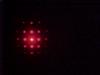
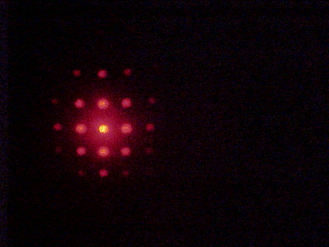
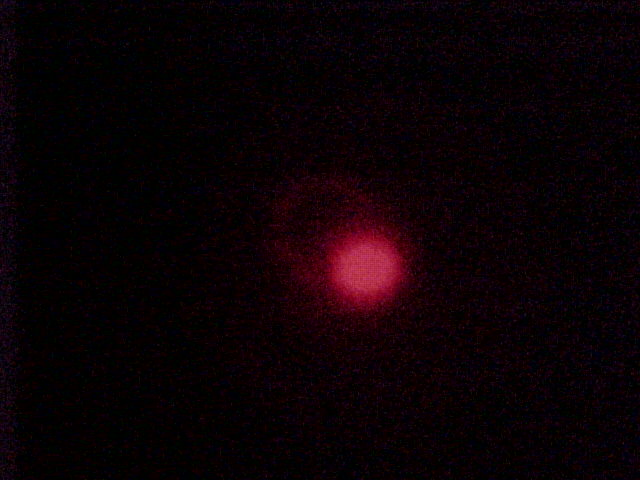
After some background reading on this phenomenon, I had a feeling that prior investigations had been a little too specific in their approach. Others had only looked at Gaussian beams coming into one specific coherent bundle. The first thing I did, after verifying the results of the others were true, was to try a non-Gaussian beam. Most of the lasers at the LTC are at least approximately Gaussian, so I needed an alternative source. I found it under the heading of "Fun Optics Demonstrations", on a posterboard hanging over the computers here. I took a diffraction lens from a pair of "3D glasses", and used the image from that. This image, and what came out when it is incident on the coherent bundle at an angle of 0 degrees, is shown on the left. Note that the output image does have more than one dot, if you click on it and look closely. The ring next to the dot looks like there was strange behavior on another dot. This was soon verified when the angle chagned. On the lower-right are two images that came out of the beam when the incident pattern was at an angle to the cable input. Notice that there are several overlapping circles, indicating that the circle phenomenon is not just for Gaussian beams.

This also suggests that this behavior is not caused by any boundary condition of the bundle. Any involved boundary conditions would be imposed by individual fibers, or the input and output faces of the cable. With just one laser dot, it was possible that it was getting manipulated on the circumference of the bundle. But now it is clear that several dots are affected independantly, so this is obviously not the case. On a related note, any observable and relevant effects of boundary conditions set by individual fibers are not likely to be involved either. Each bundle has several thousand fibers in it, and they are so small in comparison to the input and output images that any boundary effects are probably negligible and macroscopically unobservable.

Soon after these observations were made, Professor Metcalf brought me a box of cables. Inside were six identical small coherent bundles from Schott, and two other non-coherent bundles, one of which was bifurcated. The first thing I did was to use the Schott cables to duplicate every observation I had made so far, with the exception of the complex pattern (the input was too small to get a complex pattern on). All results were identical, contributing to their validity. One thought that had crossed my mind was whether or not this phenomenon was limited to coherent bundles. To test this, I tried shining laser light on the input of both noncoherent bundles. When the beam was straight on, each one emitted an image that roughly looked like a few superimposed Gaussian dots. They were seemingly random, not in a rectangular array such as in a Hermite-Gaussian mode. The bifurcated bundle's dots were very close, and almost appeared to be one. When I tilted the laser beam, creating an angle of incidence greater than zero degrees, I saw precisely what I had suspected. Both bundles had the same kind of behavior as the complex image incident on the coherent bundle. Each little dot became a little circle, which grew, as the angle increased. Thus, I have shown that this behavior is not limited to coherent bundles.

Another effect worth noting is that if light going into a bundle is linearly polarized, it comes out unpolarized. There is an explanation for this that is better illustrated if we consider linearly polarized light going into a single fiber. The light coming out of a single fiber will come out linearly polarized, but in another, arbitrary direction. This is due to the bouncing around of the photons inside the cable. It may be convenient to think of the photon as rotating, even though this is not really accurate. If we expand this view to a few thousand fibers, each one with a different and seemingly random output polarization direction, we can see that they will all effectively cancel out, and result in unpolarized light. A helpful analogy for understanding this is the atomic explanation for ferromagnetic materials. Each atom has a magnetic moment in a specific direction. In non-ferromagnetic materials, they are in random directions, and cancel out. Thus, the material produces no net magnetic field. This is analogous to unpolarized light. But in ferromagnetic materials, the magnetic moments of the atoms line up, and produce a net magnetic field. This is analogous to linearly polarized light. If you shake, rattle, bang up, or otherwise greatly disturb a ferromagnetic material, it can lose its net magnetic field, because the atoms bounce around, and their magnetic moments no longer line up. This is analogous to what the fiberoptical bundles do to the linearly polarized light: each photon bounces around differently, just as each atom gets knocked around differently, and any special orientation is lost.

The Red Diode Laser Output

This part has been removed due to an error in the data

The Schott Coherent Bundle Output

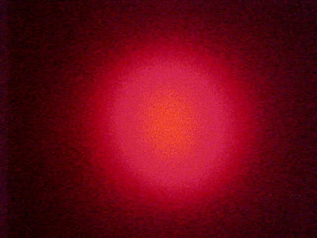
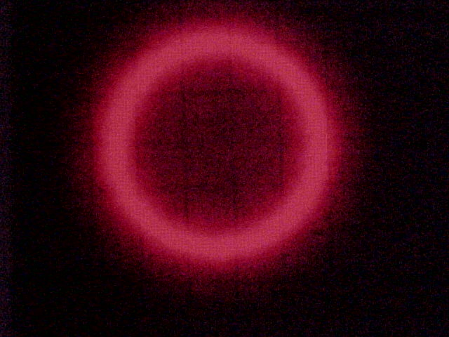
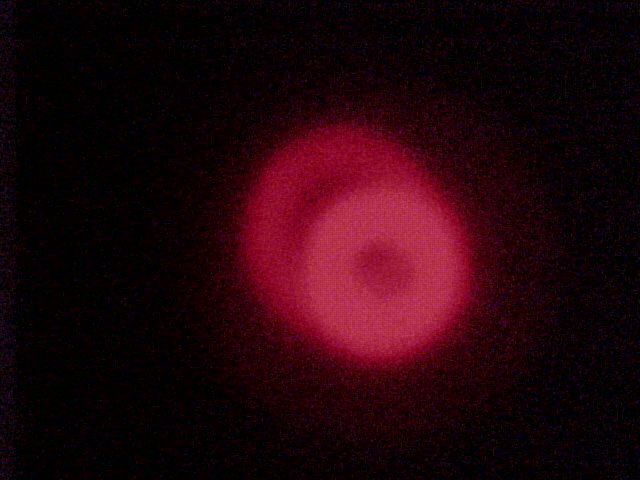
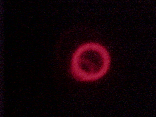
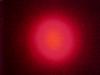
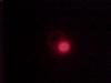
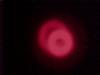
The Schott cable, model LB4453, is a coherent fiberoptical bundle, as explained above. Its opening is 0.076" in diameter, and it is 69.49" long. At right, you can see its cross-section and the corresponding 2D intensity plot. To generate the picture, I shined the red diode laser at an angle to the input of the Schott cable, and pointed the output directly at the recording apparatus. The apparatus, as discussed above, was one piece of paper, a lens, a polarizer, and then the CCD array.

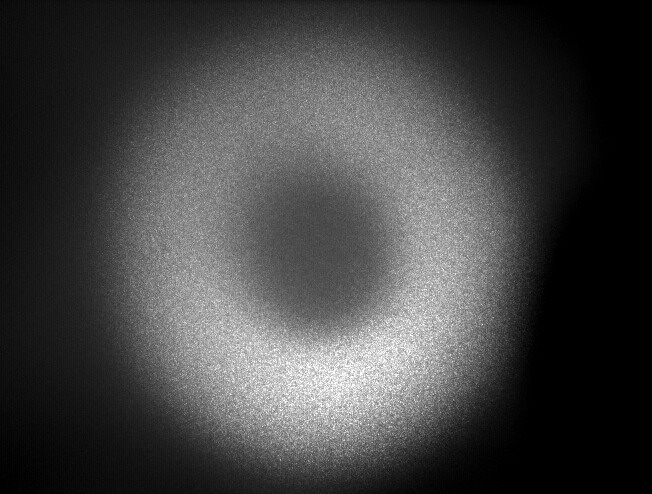
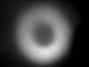
On the left, you can see the surface plots, which were made the same way as the ones for the direct beam from the red diode laser. These surface plots nicely illustrate the hollow beams that are generated from the Schott cable.

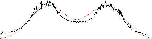
Just as with the direct output from the diode laser, I have attempted to generate best-fit functions for the transverse mode plot. Two students at the LTC in prior years have believed it to be two superimposed Gaussian plots and two superimposed Lorentzian plots. Below, I show the fit with superimposed Gaussians on the left, and superimposed Lorentzians on the right. As you can see, the fit is poor with the superimposed Gaussians, but fairly good with the superimposed Lorentzians. I plan to investigate the possibility of other functions, such as a Laguerre-Gaussian function, although that is unlikely.

best-fit, or lack thereof, with two superimposed Gaussian curves

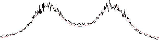
best-fit with superimposed Lorentzian curves

TODO: LORENTZIAN FUNCTION